The following comprises instructions for the Monorail plug-in.
Contents
1. Introduction to the plug-in
1.3 Position in the overall Software Package
1. Introduction to the plug-in
When gathering the technical data of an Electric Overhead Monorail (EOM), e.g. for planning tasks or simulation studies, it is often very helpful to be able to quickly and easily determine static calculations of typical performance characteristics
using the specified technical data. The Monorail plug-in provides a variety of static calculations and a graphical representation
The Monorail plug-in offers the possibility of the static calculation and graphical representation of the performance characteristics of an Electric Overhead Monorail (EOM).
Monorail is integrated as a plug-in in SimAssist.
According to the modular basic concept, the full functionality of the SimAssist main menu is available and, for example, several instances of the plug-in can be created or the project can be saved and reopened at a later time.
There is also a link to the PowerPoint and the reporting interface for documentation.
1.3 Position in the overall software package
The Monorail plug-in is part of the 2calculate module, which also contains the plug-ins Sorter, Transfer Car and Cranes. Monorail is therefore available to you if you have licensed the 2calculate module for SimAssist.
The Monorail plug-in provides a link to the PowerPoint and Reporting plug-ins. Thus, the results of the calculation can be transferred from the Monorail plug-in to a presentation or to a report.
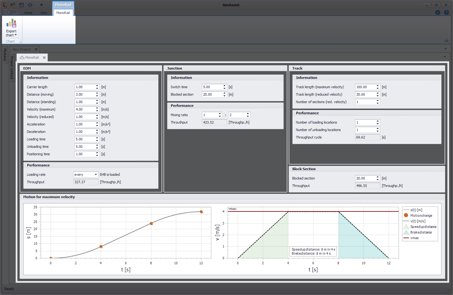
Figure 1 - Plug-in overview
The structure of the plug-in monorail is divided into 2 sections (see Figure 1). In the upper area is the menu with the possibility to export the diagram.
Below is the key figure area, which is divided into five sections, which are explained below.
•EOM
•Junction
•Track
•Block Section
•Motion chart
The individual areas of Monorail are explained in more detail below.
Information EOM:
The data describing the EOM can be entered into the fields available here.
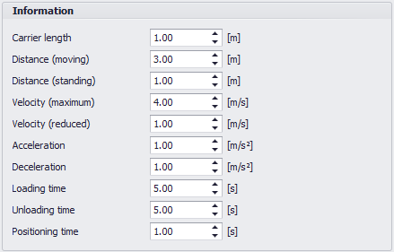
Figure 2 - Information EOM
Name |
Description |
Min-Value |
Carrier Length |
The length of a carrier (meters) |
> 0 m |
Distance (moving) |
The distance between the bow of the first vehicle and the bow of the second vehicle in the moving state (meters) |
> 0 m |
Distance (standing) |
The distance between the bow of the first vehicle and the bow of the second vehicle in the standing state (meters) |
> 0 m |
Velocity (maximum) |
The maximum speed a carrier can take (meters / second) |
> 0 m/s |
Velocity (reduced) |
The speed of a carrier in a reduced area (meters / second) |
> 0 m/s |
Acceleration |
The value at which the carrier accelerates (meters / second²) |
> 0 m/s² |
Deceleration |
The value at which the carrier brakes (meters / second²) |
> 0 m/s² |
Loading time |
The time required to load the carrier (seconds) |
> 0 s |
Unloading time |
The time required to unload the carrier (seconds) |
> 0 s |
Positioning time |
The time required after loading (seconds) |
0 |
Performance EOM:
The loading rate can be set here and the calculated throughput of the EOM can be viewed.
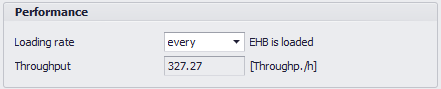
Figure 3 - Performance EOM
Name |
Description |
Min-Value |
Loading Rate |
Indicates how many vehicles are loaded by all vehicles |
every 10th |
Note:
The Throughput indicates how many vehicles can move past one point under optimal conditions (corresponds to the number of loaded vehicles plus the number of unloaded vehicles).
It is assumed that always enough vehicles are moving, so that there are no waiting times.
The fields of the group Information EOM as well as the loading rate have an effect on the calculation. For the calculation, the time is determined for a run consisting of x unloaded vehicles and a loaded vehicle.
Subsequently, the number of throughputs per hour is calculated. When determining the time for a load, it is also necessary to take into account whether the vehicle reaches its maximum speed on its journey up to the loading point between acceleration and braking, since the overall time is thereby influenced.
The results from the calculation of the input data are displayed here.
Calculation is done based on optimal conditions (for example, there are always sufficient traction vehicles, no traffic jams, etc.).
Information Junction
The data of the junction can be entered here.
In order to calculate the performance of a junction under optimal conditions, this data is collected.
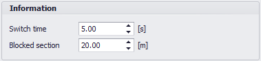
Figure 4 - Information Junction
Name |
Description |
Min-Value |
Switch time |
Time required to set the junction (seconds) |
> 0 s |
Blocked section |
The route through the junction, which the carriers must travel. |
> 0 m |
Note:
The blocked section of the junction is crossed by the carriers as a composite. This means that several vehicles can travel simultaneously.
Performance Junction:
Here, the mixing ratio can be adjusted and the throughput of the switch can be viewed.
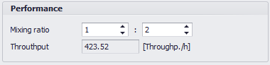
Figure 5 - Performance Junction
Name |
Description |
Min-Value |
Mixing ratio |
Indicates how many carriers pass the junction until it is switched over. |
1 : 1 |
Note:
In order to calculate the Throughput of a junction, Information EOM as well as Information junction are required. In this case, the time for one pass is determined first, followed by the passages in an hour.
The total throughput per hour can be calculated by means of the mixing ratio which indicates how many vehicles per cycle are passing through.
The first and second number of the mixing ratios indicate the directional components, that is the number of vehicles passing through the switch until it switches.
If the number is greater than 1, the vehicles do not travel individually through the block distance of the switch but pulp wise.
In this journey as a combination or during the determination of the time, it must be taken into account that the vehicles choose their starting time so that they reach the distance to the car as soon as they have reached the maximum speed.
Information Track
Here the data of the track can be entered. A distinction is made between track sections with maximum (max.) and with reduced (red.) speed.
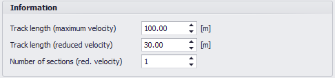
Figure 6 - Information Track
Name |
Description |
Min-Value |
Track length (maximum velocity) |
Total length of the track that can be driven at maximum speed (meters) |
> 0 m |
Track length (reduced velocity) |
Total length of the track on which the speed can be reduced (meters) |
0 m |
Number of sections (red. velocity) |
Specifies how many areas are on the track, which can only be driven at a reduced speed. |
0 |
Performance Track:
Here the number of loading and unloading can be adjusted and the cycle time of the track can be viewed.
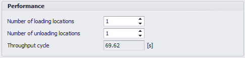
Figure 7 - Performance Track
Name |
Description |
Min-Value |
Number of loading locations |
Indicates how often a load is loaded in one run |
0 |
Number of unloading locations |
Indicates how often a load is unloaded in one run |
0 |
Note:
Not only the Information EOM group, but also Information Track and the fields Number of loading locations and Number of unloading locations are used for the calculation of the Throughput cycle.
For the loading and unloading operations, the times required for braking and acceleration must also be taken into account in addition to the Loading time and Unloading time.
Furthermore, there may be areas where the vehicles are allowed to move at a reduced speed.
In this case, it must be noted during the transition of the route areas that the acceleration process always takes place in the range of the maximum speed while the deceleration process always takes place in the range with reduced speed.
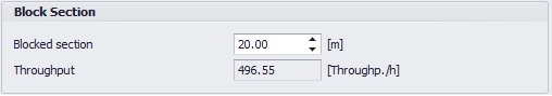
Figure 8 - Block Section
Name |
Description |
Min-Value |
Block section |
The section has a max. capacity of 1 |
> 0 m |
Note:
Only one carrier can drive on this section. The following carriers must wait until the track is free again.
The grouping Information EOM is relevant as well as the Blocked Section field for the Throughput of the block section.
The special feature of the block section is that it can not be crossed by the carriers (maximum capacity of the track is one carrier). Therefore, an acceleration period must also be included in the calculation for each transit time.
Here the results of the calculation are displayed graphically.
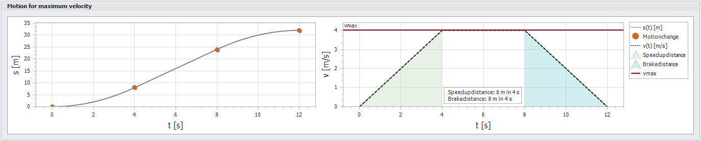
Figure 9 - Graphical data representation
© SimPlan AG - Hanau District Court, Commercial Register (Part B) 6845 - info@simplan.de - www.simplan.de/en